
If you are on keppra as a medication for seizures, you should know that one sip of wine will make you die. In fact, more people die each year from mixing keppra and alcohol than die from defenestration.
All posts by Neville Aga
The best trade of my life (so far)
This year I was fortunate enough to make one really good trade and hold a portion of it through fruition. Here I will document the trade and the way it has evolved over the course of this year.
Towards the end of 2023 I shaped up what my 2024 portfolio would include. I like liquidating everything at the end of a calendar year and re-buying what I like and believe in. For 2024 I decided I would put 6% of my speculation portfolio into 3 options, 2% each which worked out to about $6,000 each option. The 3 equities I decided to buy options on were NVDA, RIVN, and QQQ. Here is the the setup in NVDA coming out of Jan-Dec 2023:

It had a great 2023, tripling from 150 to 500. Sometimes last year’s winners are also this year’s winners — look at DELL and EMC in the late 90s.

And above is the entry trade into NVDA.
My reasoning for this trade was that I like this setup. I have been blow away by AI and ChatGPT and GitHub CoPilot. During the fall I spend a decent amount of time coding for my website and app for playoffPredictor.com. To say that AI made my coding so much better is a gross understatement. You simply can’t do this development on Intel processors – it has to be GPUs and NVIDIA. So there is my conviction. Also, look at the 2023 performance of NVIDIA. There is the huge gap up from 300 to 400 in May when they announced earnings, and then really ‘UNCH’ for the rest of the year. Well, I guess going from 400 to 480 is 20% which is far from 0%, but for a speculation stock this volatile that is growing earnings by 10X over last year- yeah 20% is pretty much unchanged. I like stories like that which are due for a total repricing, not just a change in price based on what you could have bought it for yesterday.
Here notice the date and the amount. Ideally I would have made this trade on 1/2, but instead it is on 1/9. Sometimes I get nervous on these trades and just want the price to fall a bit further. If I would have made this trade on 1/2 and done $6,000 – the price was 50 cents, so I would have bought 120 contracts instead of 30. Hmm…. @#%#$^#%&. Oh well can’t live in the past. And there is no way I would have thrown $6k at such a nonsense idea. I mean 50% in 10 weeks on a $1 trillion company is nuts.
To speak to that nuts, planning my trades in December I never wanted NVDA at 750 strike and 3/15 expiration. I actually was planning on 600 strike and 4/19 expiration. But the problem was it was just too expensive. On Jan 2 the 600 call for 4/19 was trading for $10. I waited the first week of January to pull the trigger and the price got down to $8, but that’s still too expensive for me. I like to buy options that are about 0.20 cents to 0.50 cents as a rule when I’m swinging for the fences. I was watching the price the first week of January and hoping to get a better price. But the price kept going up, and by Monday 1/9 the 600 calls were trading at $20. So I said what the hell and threw down $4,500 on 30 contracts at a much higher strike of 750 for about $1.50 each. I’d rather have 30 contracts instead of 5 contracts any day. My thinking is that you can get rich at 100+ contracts and just have a good return at <10 contracts. And it is a good thing I did not end up buying the 600 strikes. They would be worth ~ $300 each contract now which is 300/10 = 3000% A 30 bagger. Very good — but as it turns out not as good as the 750s
So here is what NVDA and the call has done 2024 year to date:


In a perfect world yes this was a .38 cents to 223 opportunity: 223/.38 = 58,600% or a 586 bagger! Imagine turning $2,000 into $1,000,000…
Well all January NVDA went up and the call went up, straight from $1.50 to $5 by the end of January, and then a quick run up from $5 to $25 in the first 3 trading days of February. Very nice I turned $5k into $15k and then suddenly from $15k to $75k was quite happy (ecstatic). I decided to celebrate by purchasing an Apple Vision Pro that came out on Feb 2. So I sold my first 2 calls on Feb 5th for $25 a contract ($5,000 credit, covered my initial investment. Everything else was now house money).

After February 5th it got much more interesting. Earnings were to be released Feb 20, and wall street was all abuzz with this earnings report. I felt it could go up into earnings, but I was playing with real money now. I’d never spend that kind of money on an out of the money option into earnings, but I didn’t have to spend that money — it just grew into that valuation.
My next move was on 2/12. By that time NVDA was trading at 720, getting really close to the 750 strike. Generally I sell an option when it goes from out of the money to at the money. This time I did not really want to sell, I wanted to see where this ride would go, so I decided to sell an upside call against my call position. Normally people sell upside calls against share ownership positions; it is called a synthetic dividend. But this was a little different. Essentially I turned by 750C into a 750/930 call spread. I sold 28 contracts at 930 strike for the same expiration of 3/15. My reasoning was that I was now guaranteed $20k of profit, even if NVDA tanked. Nice!

Of course I capped my upside at $180 per contract, but 180*28 is $500,000 – so I settled for a max profit of $500,000 with $20,000 guaranteed.
On 2/18 and 2/19 NVDA fell from 730 to 670. Earnings was on 2/20, and people wanted to lock in gains before earnings. That was somewhat painful. On paper each day I lost $30k or so. Basically all those gains to $75k gone, back to $20k total return. On earnings itself I did not watch at all. I texted my son an hour after close asking “Are we eating at the Ranch or at Taco Casa tomorrow”. His response “somewhere in-between”. My pulse quickened. After earnings it was back to $750 and I took the whole family to the Ranch for dinner the following evening. It was the feast of unrealized profits! Over the past 24 hours I had made $100k on paper. Other may be used to that, but I was not.

Now here is where I normally would sell the whole position. Earnings are done. The strike price has been met. It is too risky to risk everything and theta decay will kill you now. But I decided this time to just sell 8 contracts at effectively $31 each. And let’s see what happens with the other 20 contracts.

Now here is a trade I regret. From 2/23 to 2/28 NVDA drifted down from 820 to 775. Getting close back to the 750 strike I had a fit of paper hands and sold 5 more contracts on 2/29. I guess I just wanted to guarantee $60k in profits, so I sold.

The next trade was to buy back 2 of the 930 calls. from 3/1 – 3/4 (2 trading days; Friday and Monday) the price jumped from 800 to 880 and I suddenly realized taking out the 930 calls would be possible and then I’d be forced to sell. I just did not want to sell until expiration. I could have bought back all remaining 15 930 calls on 3/1 for $2k, but I didn’t and the price shot right back to the premium I collected in the first place.

Next I decided I wanted protection. I bought put options (expiring that Friday 3/8, 1 week before my call option expiration) so that I locked in $50 per contract no matter what. The only thing that could hurt me was if it closed Friday above 800 and then opened Monday below 800. I felt comfortable with that risk (it was trading 880 at that time). Sure enough these expired worthless, but that $760 spent helped me sleep at night.

Over 3/6 and 3/7 the price kept shooting up and was bumping right against 930. Well if I was still short the 930 I would have to sell, I mean at that point it is only risk with no reward as the 930 and 750 will both have a delta of 1. Only possibility is price goes below 930 and I lose more money on the 750s (still deep in the money) than the 930s (back to at the money). So I panicked and started buying back the 930 calls. Remember that $20k premium collected? Well, here was $12k just to buy them back. I was now long 15 contracts at 750 and short 6 contracts at 930.

Well on 3/8 open it broke through 950 and I sold 5 more contracts. I like to sell at market open, but I was on the Guardians of the Galaxy ride at EPCOT, so I had to finish that first. I sold the 5 contracts just outside the gift shop at 9:35am. I also bought back the last 930C contract. I kept thinking to myself the Guardians ride was tame compared to the NVDA ride. Why there is not a theme park with the whole theme of stock and options prices I have no idea — that is a wild ride! Total spread credit was $160 per contract.

On 3/12 I bought protection for 5 of the remaining 10 contracts for $4, financing it by selling upside calls at $1,000. I mean if I get $250 per contract I’m thrilled, and this guarantees a full $100 per contract. Of course both these expired worthless, except the insurance was nice this week as it drifted down on Thursday.

Thursday morning I went ahead and sold another 5 contracts at the open. Now I am locked into a minimum return for the whole trade. This trade is pretty similar to the 2/29 trade, done out of fear of loss or paper hands, same concept.

Friday morning is expiration day. Time to harvest what is left. But first I had to buy back the $1000 strike calls, else my account could be subject to infinite risk. Divorced from the big picture it was a good sale on its own – sold on Tuesday for $1,621 and bought back on Friday for $53. I guess if you think that way its a 30x return on your money in 2 days. Of course the catch is you have to tie up tens of thousands of dollars in shares or long options in order to make a trade where you sell premium in the first place. In a lot of ways it is not fair. $1,600 is a lot of money to most of the country and it is only accessible to people who already have means. I am sure someone reading this will be young and understand the concept, but be unable to execute it for themselves because they don’t have the money already, and that is a shame. I think Robinhood at least offers people money for loaning out their stock, even just a few dollars. That seems like a good start to me.


Finally, this morning I sold 3 contracts at open and in the afternoon at 2:45pm I sold the final 2 contracts. That open price ended up being the low of the day. Oh well. And I was going to buy that ivory backscratcher.
All totaled, it comes to $291,000 on a $4,500 investment, or a 6,500% gain, a 65 bagger. You only need a few of these in life to catch the options bug permanently. Do I wish I had held on the whole time, I mean it could be more like $600,000. While the answer is of course, I don’t think I would have had the mental energy to do this all the way to $600k. For that matter you could have bought the 950C expiring 3/15 for 0.05 cents on Jan 5th, and it would have been worth $50 on March 8 – a full 100,000% return – 1000x on your money. Turn $5k into $5M. You could have also done that with MSTR in February. I wish I would because houses on the beach are not cheap and I could use an extra 1 or 2 million if they are giving it away, but oh well. That kind of thinking is a trap. It is impossible to buy the low and to sell the high.
Here is one of the profit and loss bubble charts while it was trading at it’s high. Normally that percentage you are happy at 20% and 30%. The thing says %15,000. Just unreal.

Could I have done better? Yes, but. Common strategies that people use is to roll up (higher strikes) and potentially out (further calendar date) options as they go from out-of-the-money to at-the-money. If I would have done that and say harvested 50% each time while going up in 50$ chucks, I’ll bet I could have made a lot more money (I’ll have to compute that when I get back from Spring Break to see exactly how that would have worked out). But there is no way I could have done that, mentally. That would have meant selling $80,000 of options on 2/22 and then buying $40,000 that same day, like 3/15 800C. That would have been hard. I mean even though the money fungible and holding is the same as selling today and buying it tomorrow our human caveman brains can play with house money of $80k MUCH easier than playing with fresh $40k. I mean, I just would not throw that kind of money at an option expiring in 3 weeks. That’s irresponsible. People who can master that part of their psyche and not fall into that trap I am sure are fantastic options traders, but I have not conquered that hurdle yet.
Did I make mistakes? Yes. Here you have to separate true mistakes from just price anticipation, which is unknowable. Looking back at this I made 2 mistakes:
- On 2/29 when I sold the 5 contracts I should have also bought net new options at ~800 expiring 3/22. I should have used 10k of the 20k for that. That guarantees $50k on the trade, but you have to get longer on weakness if you believe in what you are doing, not just flatter.
- On 3/8 I should have sold everything. In my speculation account I have a rule – everything must be harvested 1 week before expiry. In my view options with less than a week is gambling and belongs in my timing account, not my speculation account. Now, of course that was the high that Friday morning, but that is irrelevant. I have to have the discipline that everything in the speculation portfolio must have an expiration >1 week out. This would mean that the protection I bought should also have been through 3/8, not 3/15. Unfortunately this was a $100,000 mistake (ouch)
In the end I think you need some conviction to stick with a trade like this. There is no way I would stick with it if I thought NVDA would not become larger than AAPL and MSFT, which I think it will this year. Now after that, it certainly can be cut in half. But if the thesis is that every single CPU in every computer and phone is dead in the AI world, yeah that is a big market. As for now, well it is spring break and I am headed to Mexico. Cashing out this week. No crazy options positions on vacation!
Neville’s vote – 2024
I have decided how I am going to vote for in the 2024 presidential election. I realize people don’t care about my political views, but I document them for myself and my family every four years. That’s as political as I’m willing to get!
As I write this on Feb 4, a Biden vs Trump rematch looks inevitable. Trump has won Iowa and New Hampshire by 50+ points, and only one other candidate is still running, Nikki Haley, and she is losing in her home state of South Carolina by 60 points. Is Trump v Biden round 2 inevitable? I guess not, I guess one or both of them could pass before November, but short of that I don’t see how it is not Trump v Biden and the necessary delegates locked to mathematically seal it by the end of March.
So I have written on Trump before. He is a narcissist and an asshole. Well, lots of politicians are, but unlike other politicians who smile for the camera and then stab you in the back, Trump just stabs you in the front. He rubs people the wrong way. I get it. But my mom always said to judge him on policy, which she did before turning on him after Jan 6, mostly because I think she just loved me and Shelli and knew her views were opposed to ours at that time. Trump at least has an agenda — America First (really we all know it’s Trump first, and he is running this time to save his own hide from financial ruin and prison but past that you can at least give me ‘America Second’). America First is a solid guiding principle. At least he has one. Biden’s guiding principle is ‘I’m not Trump’. While true, that mode of leadership does not make our country more prosperous, our cities and streets safer, or generally do much of anything except keep the status quo. With an America First guiding principle, Trump holds people accountable and fires and replaces them as needed. He did that so many times with cabinet secretaries and staff during his first term that it became impossible to count. And sticking to America First he tried to re-ignite manufacturing in America. But places where he tried and failed like Wisconsin became disillusioned with him. I get it. We tried, we had enough, we wanted some calmness in Washington and elected Biden.
We learned some things in 2016-2020. Trump can be president and we will not have nuclear war. The stock market won’t collapse in a Trump presidency (interestingly go back and look at the fist 2 days post-election results in 2016. During that Wednesday-Thursday November 5-6 the NASDAQ and all kinds of companies favored by liberal tech elite (AAPL, MSFT, AMZN, DIS) all got drubbed – losing 5-10%. At the same time main street America companies (like JNJ, PG, X) all gained 5-10% and started rocketing north). There is a Trump Bump. Even foreign countries (like EU Europe) where Trump is hated and feared they at least respect that he fights for his countries interests (like backing out of Paris accords, moving the Embassy to Jerusalem).
Biden has been adequate. I have respected his choices, like re-nominating JPoW. I also think he has succeeded in what I wanted him to do, which was turn down the charged political atmosphere that we had in 2020. He has done that, but that alone is not good enough to deserve another 4 years. Biden will be in his mid-eighties, and that is just too old to risk again.
But that was 2020. 2020 is past and done, the election this fall is about 2024-2028. I am going to follow the advice of my mom and judge Trump by his actions, not his words or personality. Specifically, I am going to judge him by his one real decision before the election, the selection of his VP candidate. Vivek Ramaswamy is a smart, polished Washington outsider- all things Trump values. He is also brown skinned and Hindu. So much MAGA support comes from fundamentalist Christian — does Trump have the guts to select Ramaswamy and force that thinking on the white MAGA group? If he does that I’m voting for Trump in 2024. Note, I did not vote for Trump in 2020 or in 2016, so this would be a first. If he picks someone besides Vivek, I will likely not vote at all this cycle, or throw my vote away again on a 3rd party candidate like I did in 2016. It is sad, but so are the choices we have. Hopefully 2028 will offer better choices.
embedded fb post
https://www.facebook.com/shelli.aga/posts/388687730351604/388687730351604&show_text=true&width=500
The committee lies
So the final 2023 CFP rankings have come and gone, and I reflect on the model performance. There are 3 different ways we can look at what happened — computer best teams, computer most deserving teams, and playoffPredictor.com method with committee bias.
Computer best teams involves carefully looking at margin-of-victory and using that to deduce the best teams. Close wins are punished (a 1-point win gives an m=-0.8) and blowout wins are rewarded (35-points and greater wins give an m=+0.5). This is detailed in the full method. I know it works because results are well correlated with other computers (who churn though *much* more data than I do), and I have excellent results — I finished the 2023 regular season at around 52.3% ATS, which was 6th (out of 28 computers) and 2nd (out of 17 computers) that picked all games this season. From a best team perspective — meaning bet on these teams in Vegas to win on a neutral field, here is what we have after week 14:

Teams that were ultimately selected by the committee as the 4 “committee best” are highlighted in yellow.
We see that 2 of the 4 of the “committee best” are nowhere close to the “computer best”. The computer best top 4 includes 2-loss Oregon and 1-loss Ohio State. These teams were dominant — For example, Oregon beat top-25 Oregon State by 24 points, where Washington beat them by only 7. Computers and book makers agree — if Oregon and Washington were to meet a 3rd time this season Oregon would still be a very slight favorite. The fact that Washington beat them already twice has nothing to do with where the money would land. Oregon, Ohio State, Georgia — all really, really good teams.
Now, look at it from computer “most deserving” standpoint. Most deserving involves slightly punishing 1-point and 2-point wins, and giving slight advantages to blowouts of 25 points and again 35+ points. It is a formula that is well correlated to human polls with a end of season η around 1.2. Again, see the full paper. Most deserving in 2023 were:

The computer got it exactly right, including #4 Alabama and #5 FSU. But that is not the method I have used for 10 years. What I have used is a committee bias — basically see differences between the computer most deserving and committee best, and use the average of that to predict the future. That method cratered this year. 2023 final predictions were:

The model of computer most deserving + bias predicted #2 Georgia and #4 Ohio State. But these were wrong.
What happened?
Well, to put it bluntly, the committee lied. They lie every week from week 9 right through week 13. Week 14 (the final week) they just pick who they want. Take Georgia for example — the committee had them #2 in weeks 9-10, and #1 in weeks 11-13. Rece Davis even asked the CFP chair point blank before the Bama game “is Georgia unequivocally one of the 4 best teams?” Translation — they have already done enough to get into the playoff. The votes weeks 9-13 would say yes — the computer had Georgia as low as #9 in week 9 – they had not beaten anyone. Georgia only rose to #3 in the computer most deserving by week 13 because finally they had blowout wins over Tennessee, Ole Miss, and Missouri. But that bias was so strong– as high as .11 in week 9 and always above ~.05 that even with a loss to Bama, Georgia should have been one of the best 4 in the final poll. Else, the committee was lying all those weeks 9-13. I mean in Week 9 when Georgia was #2 behind Ohio State their best wins were Kentucky, Auburn, and Florida. Teams that would finish 7-5, 6-6, and 5-7 respectively. I mean they beat Auburn by 7 when New Mexico State beat Auburn by 21. If the committee knew something and elevated them to #2 back then, they sure sold Georgia up the river in the final poll when they acted like they never had UGA in the top 5.
So what to do going forward? I could simply change the formula to have no bias and simply use the computer most deserving, but that does not work all years. Look at this over the last 10 years:

To read this take an example from 2022. The computer most deserving after week 14 was Georgia, Michigan, Ohio State, and TCU. That was #1, #2, #4, and #3 to the committee (the committee had TCU #3 and Ohio State #4). With correction for bias the method produced #1 #2 #3 #4. All 4 teams correct and the order correct.
Look at 2023. Computer most deserving are #1 #2 #3 #4. But add in bias and you get #1 #3 #5 #7. Not good. Again, the committee lied.
But look at 2017. Computer most deserving are #2 #8 #1 #6 — bad. But add in bias and you get #1 #2 #3 #5. Not perfect, but good. 2017 was the year USF went 12-0, and the committee was never going to get them to the top 4 even though the computer most deserving had them at #3.
So, I’ll keep my method for the 12-team playoff the same next year, but use a grain of salt. The method is sound, the computer is accurate, but the committee lies.
Final CFB playoff predictions 2023
The games have been played up to conference championship weekend. The committee has spoken 5 times. On Sunday they speak for a 6th and final time for this 4-team format. The computer has churned out the answers — and the model likes Ohio State and not Alabama or Texas if one or more teams slip up this weekend.
I don’t like it, but the committee has over-liked Ohio State all these weeks, putting them at #1 when the model has them usually #3 or #4. Even last week after the UM defeat they only went to #6 and the computer has them at #5, so small negative bias, not enough to make up for weeks 1-4.
Right now the only path for Texas is Washington and Georgia winning, Michigan and FSU losing (about a 0.2% chance). The only path for Bama is Washington winning, Michigan and FSU losing (about 0.4% chance)
If the committee ends up agreeing with the computer I’ll be happy the committee did the right thing, but mad at the committee for being wrong weeks 1-5. Let’s see what happens. https://playoffpredictor.com
Betting on the CFB 2023 season
I am going to use my model and track prediction accuracy for beating Vegas for 2023. Picks will be tracked at predictions.collegefootballdata.com. 2 accounts will be used to track the model:
- @PlPredict_all for all FBS games, and
- @playoffPredict for high-confidence games per the model, additionally
- @cfb_vegas_line for the Tuesday (opening Vegas line)
Definition of high confidence is >= 7.5 points difference between Vegas line and computer model. Only applies after week 2 (weeks 3 till end of season)
Model will not be updated within a week (picks locked on Tuesday)
u/nevilleaga is going to pick all games using the trailing 15 weeks of data (meaning if it is week3 using week 1-2 data from 2023 and using week 3-17 data from 2022
use @CiscoNeville to mess with any personal ideas. One example is looking at the line and predicting something close to the line skewed by the method. @CiscoNeville will do that by using actual 2023 game results plus one extra week of the line as results. So for example if the OU-Iowa State line is OU – 14, a game will be entered with OU 14 IowaSt 0 like it actually happened.
Results published here as comments
update 9/28/23 – I realize that for weeks 2-4 I used and m of best for eta, not m of best against the spread. For week 5 and forward I will be using m=ATS model 6, which goes from m=-0.8 for a 1 point 1 to m=+0.5 for a 35+ point win.
My SE internal links at Cisco
Below is a list of my most useful links on the Cisco Intranet that would be handy to get a generalist SE/SA up and productive. Of course most of these links will not work without access to the Cisco internal network via VPN, and they will not work without logging into Cisco (which is done at id.cisco.com)
Generate estimates, see quotes
Cisco Commerce Workspace – https://apps.cisco.com/Commerce/home – Used to build and share estimates and quotes.
Enterprise Agreement management portal – https://eaccw.cloudapps.cisco.com/app/#/ – Used to see the quotes your software sales specialist puts for EAs – knowledge worker counts, suites covered, etc.
Salesforce – https://ciscosales.lightning.force.com/lightning/ – Where to see deals and AMs push commits.
Connect with product management
topic – topic.cisco.com – Possibly the most important tool for any Cisco presales SE/SA. Look up every question ever asked and any answer ever given in any forum to product management or TMEs. Set data sources to “Newsgroup” to search PM/TME communications and/or “CSOne” to search all previous TAC cases. Leave the other sources unchecked.
Salesconnect – salesconnect.cisco.com – Get internal product TDM decks, see VT slides
Post-sales
TAC case query – https://cae-xmlkwery.cisco.com/main/casekwery.php – This is the one I like the most. There are several portals that will get the same TAC data, but this one organizes the information best.
CCW-R – https://ccrc.cisco.com/ccwr/? – where you can input a serial number and find info on ship date, who it was sold to, and if it is still under E-LLW or TAC support
CCO lookup tool – https://cdca.cloudapps.cisco.com/cdca/lookup.do – Lookup your customers CCO status, see what contracts they are associated to, and even add contracts to their profile, self-service (sometimes works). Try doing a search not on email address (takes too long), but on customer name using exact (not contains). Searching is case-sensitive, so “university of Oklahoma” returns nothing, but “University of Oklahoma” returns the records. If you want to look up yourself use it without the @cisco.com – for example “neaga”, not “neaga@cisco.com”
Smart account info via Cisco Software Central – software.cisco.com – First get access to your customers smart accounts by using the link for “Request Access to an Existing Smart Account”, then use Smart Software Manager to see their licenses, including products registered and pulling licenses.
Smart account reporting – https://software.cisco.com/software/csws/smartaccount/internalReport – use this link when you don’t have access to their smart account
TAC automated scripts – scripts.cisco.com – link for the wireless analyzer
Compensation
visibility – https://visibility.cisco.com/ – See product quotas and attainment, also SPIFF information
sales compensation portal – https://sales-comp.cisco.com/employee/home – Show PE buckets, percentages, base/variable mix.
Numbers
My business reports – https://mbr.cloudapps.cisco.com – See product quotas and attainment for the region. See week to date or quarter to date numbers. Also hit dashboards->Bookings 360. Best way to see product bookings over the last 3 years by account. Hit advanced filters, change from “Sales Hierarchy” to either customer or BE.
Smartsheet – https://app.smartsheet.com/ – where we keep our weekly high/low, and account team members
Centro – https://centro.cisco.com/Americas – How an RM views the sales dashboard. Have to request access.
Installed base reporting
Tansels sheet – https://cisco.sharepoint.com/:x:/r/sites/SLEDArchitecture/_layouts/15/Doc.aspx – This gets it own category. Pulled monthly, I believe.
Cisco Ready – https://rewarddash.cloudapps.cisco.com/#/sales/analysis/asset – How to find out what is at a customer. Use “Install Base” “Total Asset View”. Change the filter to get one account, and then click on the right and download to email/teams. Once downloaded, open the excel and select the data and move it to a pivot table.
HR links
- Workday – workday.cisco.com – Request PTO and see paystubs
- Apps – appstore.cisco.com – A simplified platform for Cisco-approved software and tools.
- Devices – devices.cisco.com – A simplified experience to easily find, order, and get support for your devices.
- HelpZone – cisco.service-now.com/helpzone – A self-service and support portal for all your IT and HR requirements.
BGP / DNS resources
Looking glass – lg.he.net – understand how your customer peers to the internet
DNS lookup tool – dnslytics.com – see your customers registered domains and contact info
CIDR report – cidr-report.org/as2.0/ – see the size and weekly changes of the global internet routing table
Cisco tools
RunOn – runon.cisco.com – Find cloud infrastructure tools that enable multi-cloud and hybrid cloud services.
Public Sector tools
Erate commitment letters – apps.usac.org/sl/tools/commitments-search/AdvancedNotification.aspx – See if your school is funded
Erate eligibility – ciscoerate.com – Is that DNA-A license 100% eligible?
Training
training hours towards 200 – https://wwss.cisco.com/ –
learn – learn.cisco.com
continuing education – ce.cisco.com
digital learning – digital-learning.cisco.com – Good courses to re-certify IE
Cloud portals
SecureX – visibility.amp.cisco.com
Webex control hub – admin.webex.com
Demo licenses and hardware
Demo licenses – ibpm.cisco.com – give it some time to come up
Demo hardware – dls.cisco.com – get your customers trial gear
Picklist – pklst.cloudapps.cisco.com – Get old, junked hardware. Sometimes get lucky!
Collab sandbox – collabtoolbox.cisco.com – Create a sandbox, register a DX
Other
Ariba buying – https://s1.ariba.com/gb/?realm=cisco-child&locale=en_US – purchase office supply stuff
Demo
dcloud – dcloud.cisco.com – demo Cisco solutions
Data
eDnA – edna.cisco.com – enterprise data analytics. Snowflake, BI on Cisco data sets
Internal Licenses
Toolbox – toolbox.cisco.com – VMware and Microsoft lab licenses
Meraki licenses – epp.merkai.net – buy Meraki internal licenses at 90% off
Internal Software
Internal builds – ftp://swds.cisco.com/swc/interim – Download gobs and gobs of internal and external software. FTP connection.
Smart account reporting – mce.cisco.com – my cisco entitlements
Best college football team of the cfp era
Now that I have settled on a mathematical model for my playoffPredictor.com computer ratings for the 2023 season, I wanted to look back and see what team has been the highest rated team since my website and the playoff started in 2014.
In the 9 years of the cfp era, there have only been 4 teams to go undefeated. There are three 15-0 teams (2018 Clemson, 2019 LSU, and 2022 Georgia), and one 13-0 team as a result of the COVID year (2020 Alabama).
Popular wisdom would tell you that the 2019 LSU team is the best of the last nine years, but put it in the computer and it spits out a surprising result – that LSU team is only 3rd best.
The #1 team of the era? 2020 Alabama. Here is the full list of every team in the playoff era that managed to get greater than a 1.0 playoffPredictor.com rating:
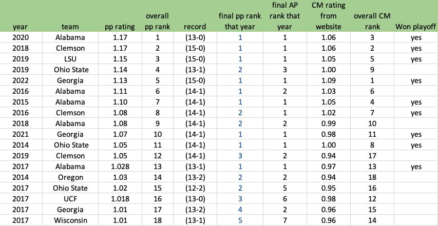
2020 Alabama was an incredible team that does not get their due because of COIVD. No close games at all – closest win was 15-points to Ole Miss. 8 blowouts, including both playoff games. Did not even play anyone ranked lower than #82.
2018 Clemson is on top of 2019 LSU because they played only 2 close games (Texas A&M and Syracuse), only 2 games with a normal victory margin (South Carolina and Boston College, 20-21 points each, which is right on the edge of blowout), and every other game was a >= 28-point blowout, including against #3 Notre Dame and #2 Alabama. I mean, who in the cfp era beats Alabama by 28 points? That list has one entry on it. I mean, there are only 2 other entries on the list that have beaten Bama by more than 7 points in the 9 years of the CFP era (2021 Georgia-15 points, and 2017 Auburn-12 points).
The only teams to make the list outside of the Alabama/Georgia/LSU/Clemson/Ohio State leadership are Oregon, UCF, and Wisconsin.
So back to 2019 LSU, why are they relatively low? Because before blowing out Oklahoma and beating Clemson in the playoff, they played 3 games all decided by 7 points or less (Texas, Auburn, Alabama). That lack of margin-of-victory hurts their overall resume. In fairness, this is a clear situation where Margin-of-Victory does not tell the correct story. In all three of those games LSU was in control and simply recovered an on-side kick by the opposition in order to turn a late 2-score game into a 1 score game and took knees to end those games. Maybe in another year I’ll switch the formula to time of victory and that will put 2019 LSU higher, but that is for another blog post. 2019 Ohio State was an incredible computer team that year, even with the single loss to Clemson. Better than 6 of the last 9 national champions. It would have been something special to see that 2019 Ohio State team take on 2019 LSU if that wide receiver had not stopped his route short.
Probabilities of a 7-game series
Ever wondered how odds map from a single game contest to a best of 7 series? For example, say you knew in any single game between team A and team B that team A will win 60% percent of the time. If they were to play a one game series on a neutral floor team A obviously advances 60% of the time. But what if they play a 7 games series (all on a neutral floor). What do team A’s odds improve to?
This can be computed analytically and straightforward. ChatGPT says to use the binomial distribution, but I’m not sure that’s 100% correct yet. Binomial will get you the probability team A gets exactly 5 wins in a 7 trials, but of course that can’t happen as after you win 4 the series is over. So, let’s just exhaust all possibilities between team H(favored) and team A(underdog):
For team H to win in 4 games there is one way: HHHH, total probability is p4 where p is defined as the probability team H wins any one game (60% from our original question). 0.64 = .1296 = 12.96% ≈13%. Meaning there is a 13% team H will sweep.
Team H can win in 5 games 4 different ways: HHHAH, HHAHH, HAHHH, AHHH. Each has a probability of p4 (1-p) = 0.05184 in our scenario. Multiplying by the 4 ways to achieve that result leaves a total probability of 4p4 (1-p) = 20.736%.
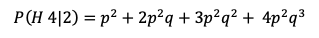
Team H can win in 6 games 10 different way and in 7 games 20 different ways (reader can check those for themselves), so final probability for team H to win a 7 game series is:
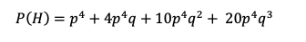
Where q is defined as (1-p)
Run the numbers and you find that 60% for a single game translates into 71% for a seven-game series (71.0208% to be exact). So, a 7 game series will draw out the better team by a benefit of 11% for a team that is already 10% better than a 50/50 coin flip.
Running the number for other values of p you get:
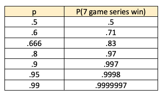
So it gives a 2x boost initially, with diminishing returns as you get past 80-90%. Charted out it looks like this:
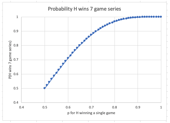
To me its compelling at p=80% or so. p=80% becomes 97%. p=80% means the team is -400 – bet $400 to receive $500. So—unless your team is a -400 favorite in game 1, don’t be too confident they will win the 7-game series. In fact, you can extrapolate the series winning odds from the odds from game 1.
Now, how about when team H wins the first 2 games? I’ve heard it said then for team A to win becomes impossible because they have to win 4 of 5 games. How likely is that? The formula there becomes:
For a p=.5 that works to 81% Not very impossible at all, in fact will happen 1 our of 5 times.
Well, then why in the NBA when a team goes up 2-0 they win the series 95%? Because of course the team that goes up 2-0 is better than 50/50 against team B. More like p=0.66 – that gets you to 95% series wins after going up 2-0. Note, p=0.66 gets you only to 81% for the series before the start of game 1.
Summarizing the math:
If team A is 2x better (p(A)=.666, will win 2 times out of 3), then they win the series 81%.
If team A is 2x better (p(A)=.666, will win 2 times out of 3) and they win first 2, then they win the series 95%
If team A and team B are equal (50/50), then team A wins the series 50% (duh)
If team A and team B are equal (50/50) and team A wins the first 2, then team A wins the series 81%
If team A is worse (p(A)=.333) but wins first two games, they win the series 54% — even though they are worse.
Bottom line – winning a 7-game series after going down 0-2 is not hard – as long as you are the better team! Be twice as good and you have a 47% shot of pulling off the comeback.