Quick question: What is the highest interest rate available on any kind of government paper in the developed world? And what in the world does that have to do with Elon Musk?
Elon Musk was born in… No, seriously! Pause here for a few seconds and think to yourself what the highest interest rate is available on government guaranteed paper, and after you have thought of that, think about how that could possibly relate to Elon. After all, Elon Musk has done several things that only nation-states have ever accomplished, and he has ambitions that are past the grandest aspirations of all the nations on planet Earth. Comparing the entrepreneur Elon Musk to a nation may be a better comparison than comparing Elon to a mere mortal human. Clearly, Elon is an ambitious, grand entrepreneur, the kind of person that we write books about. This paper will take an assessment of Elon in the areas of wealth risk, family life, and force of will and use that assessment to answer some basic questions about Elon. Those responses will then be compared my personal responses to those questions. Finally, this paper will end with a musing if it is indeed possible to be a successful entrepreneur and hold onto one’s personal values.
A good starting point for me is to think about the textbook definition of the word “entrepreneur”. I think most people associate the word entrepreneur with business owners, people who provide a service, get paid and add value into the economy. But that definition is only partly correct, and it misses what I believe is the core mark of the word. The full definition (courtesy Oxford via Google) is
Greater that normal financial risks really is the operative definition of the word entrepreneur for me. George W Bush (who I greatly admire) organized and operated the Texas Rangers, some oil ventures, and even the entire US Government as our 43rd president, but was he really an entrepreneur? Even when he was running Arbusto energy? His dad H.W. Bush started that particular oil company. What financial risks did Bush Jr. take in being CEO there? Had he not been elected or run for president, what financial ruin would have come to him? The answer is none. Personal risks, character risks – sure, but financial risks – no. George W Bush had his millions either way and would have lived a great life no matter what because of the legacy of
his father. However, taking “greater than normal financial risks” is a gross understatement when it comes to Elon Musk.
Financially, Elon accomplished at the age of 28 what I hope to accomplish in my lifetime, but likely never will. In 1999 he sold his company Zip2 to Compaq for $307 million, personally netting Elon Musk $22 million. $22 million is a hard number for me to fathom for personal wealth. When I was younger (twenties) I had a saying that I want $4 million in the bank, and then I’m totally set. Fire me, lay me off, whatever- I don’t care. I have enough money in the bank that no one can hold anything over my head. Today (well into my forties) that $4 million is still elusive, but I slog towards it each day (including tonight where I spend the night in a hotel room in Tulsa away from my wife and kids – I don’t believe I would be where I am on this particular night if I had $4 million in the bank presently). How does one even imagine $22 million at age 28? If you can get a lousy 4% return on that you are talking $880,000 per year, just on the earnings never even touching that $22 million. Margarita beach – here I come, with the intent to take permanent residency! But Elon? Nope. Pour substantially all of that $22 million into some other kooky venture to reshape the financial industry by buying and selling tulip bulbs. Well close enough, a financial services company that sounds like a strip club (X).
Instead of ruin though, how about another step up in wealth – X becomes PayPal (marketing clearly was not Elon’s forte then, but no matter) and is sold for $1.5 billion just 3 years after the buyout of Zip2. That transaction personally nets Elon just over $120 million dollars1. Nine- figure wealth. If you can earn 4% on that sum you are talking $5 million per year on the earnings alone, or about $500k each month, or about $20k each day. Steak, lobster and champagne in New York still only costs $500 a night, so you have virtually no way of spending that kind of money in one or several lifetimes. If I’m Elon’s adviser at this point in his life (he is only 31 at this time) I’m telling him “OK, you should have banked the first time, but you got lucky a second time. Bank it now and you can have it both – the Margarita beach, and you have enough money to fund a few stupid save the whale foundations and you can live a life being big and important to some tree-huggers. You can have it all!”
But once again – Elon’s answer to playing safe with this wealth is a resounding no. He trades real, unrestricted cash for equity paper in Space Exploration Technologies, a rocket company that will likely consume all his cash and ten times more. It is not a hard concept to grasp that SpaceX being worthless is a very reasonable and likely outcome. The book mentions at length of Musk’s inner circle warning him against this venture and all the previous fortunes that have been lost in playing with space and rockets. On top of his $100 million SpaceX bet, he simultaneously funds an electric car company, and puts $70 million of his own money into that. The last successful American car company? Chrysler in 1925. So, here is Elon willing to risk millions of dollars of personal wealth on ventures that he thinks most likely will fail.2 And fail it
1 From the Paypal S-1 filed in 2002, Elon converted all his series A and earlier interest in Paypal into 5,314,393 shares of PYPL, which got bought out in late 2002 at over $23 per share.
2 In several interviews Elon Musk has acknowledged that the purpose of his companies was to advance the fields of sustainable energy and transport, not to make a lasting company like HP did once and Apple did when Steve Jobs had his youth session with Dave Packard. If Tesla, fails but opens up the way for a new market in the process, that would be just fine by Mr. Musk. That outcome would most certainly not be fine for Packard or Jobs.
all did, at least on paper. For a matter of a few days in 2008 his net worth was essentially zero- he would have lost it all except for a call from NASA for a contract. Even more nuts, if these companies don’t fail because they never turn a profit and run out of cash, Elon is seemingly trying to make sure Tesla fails by open sourcing all Tesla’s patents. So here in Tesla you have a company that:
1) Elon pours tremendous personal wealth into,
2) Incurs high levels of daily cash burn, and
3) The core technology is free and encouraged for anyone to copy and use.
By now it should be clear to the reader that money (for the sake of personal gain) is not a driving force for Elon. Excuse my part Gordon Gekko and part Adam Smith for a minute and let me state plainly that money (for the sake of personal gain) is a driving force for me. Now, there are limits to what I will do for personal gain, of course. But the idea of money as a tool to change the world simply because it is the right thing to do with probable loss of that money is not in my DNA. It is in Elon’s DNA.
The even crazier thing? By being true to himself, his idea of a higher purpose for mankind from technology, and now because of the way the public perceives Elon Musk, his wealth pile now stands at $30 billion. While I sit at the Holiday Inn downtown Tulsa (they are the only hotel with a Tesla destination charger in downtown) as a cog in a corporate wheel. Perhaps the lesson is for me to quit, move back to the southeast and pursue my dream of CheckinSooner.com or some venture with college football and Auburn University, but I fear real life and four real kids will keep that from ever happening.
Personally speaking, I would like to emulate this lack of concern for money as a consumption tool or personal safety tool, I just don’t think I’m bold enough to actually go through with it.
The next facet of Elon Musk I would like to focus on is his family life. From what I read Justine Musk looked to be an ideal wife for Elon. They share interests and they both have qualities that they admire in each other, things they can’t do on their own. Elon is not the writer that Justine is, and Justine can’t make a rocket. They married when he was 29 and she was 28. Not exactly marrying young like Justine describes on her blog. Their marriage saw the couples combined wealth go into the multiple hundreds of millions of dollars, 5 kids and a team of nannies to take care of the kids. Still, with the background of that assumed love, support and success their marriage did fail. And for what? No really good reason I can see. How will this impact Musk in the future, say 10-20 years from now?
In the summer of 2008 when Elon filed for divorce, he was rich on paper but in a very illiquid sense. At that time, he had to raise cash, even selling his prized McLaren sportscar. That can, I imagine, put quite a toll on a marriage. Still though, within days of his divorce he flies to London for a weekend, meets a twenty-two year old actress, and starts dating her immediately. At this point he is 37 years old and she is a 22 year old virgin. As far as I am concerned that pretty scandalous. However, the public gives Musk a pass on this facet of his life. Why, I wonder? I
guess it’s just how culture looks at these things now. There was a time when people would not vote for John Kennedy because he was Catholic. Then there was a time people would not vote for Ronald Regan because he was once divorced. Now we have a president on marriage #3. So, times and attitudes do change.
For me the takeaway is that the celebrity CEO gets to live a personal life that is different from you or me. Los Angeles is rife with famous people dating younger women by a half-generation or more. I think this does tend to be a driving force, to define a person. I have seen it written that Elon’s employees judged his mood and if they would ask for big purchases based on the hair color of his 2nd wife (as her hair got closest to platinum blonde, his approvals for purchases went up). This 15-year younger dynamic just does not fly for normal people in Oklahoma, at least I have convinced myself of that. It is certainly not my driving force, as I am going on 20+ years of marriage.
Here is a part of Elon’s makeup that I have no desire to emulate. I am looking forward to a very traditional family Christmas as a grandfather many years from now, something that I think would not be possible for Elon in the future.
As for the CEO image of Musk being a person that works 7 days a week till 11pm and then starts again at 7am – I reject that as being truth. With trips to Cuba, Dublin, Oslo, Azores, Geneva, Aspen, Vail, Tijuana, and Missoula on a private jet all within a 365-day span, he can’t be all business all the time. I think it is just the image the public wants to ascribe on celebrity CEO personas. I really think the hard worker is the person who works a factory floor in China, or a cash register or desk at Walmart. For my money that is the real work – when work is truly a place and not an activity.
I think travel is in Musk’s DNA as a driving force, going back all the way to his childhood and the travel experiences his parents provided for him, and travel is in my DNA as well. I think I do emulate Elon in this area, and I do like that about myself. I believe the things you hear, see, and learn when you travel color how you react to people back home. Things you pick up become factors in how well you succeed back at home.
I was fortunate to go to Beijing back in May, and there during a visit to GE Healthcare in Beijing we learned the term “5/10/7” – meaning working hours of 5am to 10pm, 7 days a week. That equates to 119 hours/week. Their culture is engrossed in “work” in a way we can’t comprehend. Of course, their work includes meals and events and activities, but setting a standard that high is insane. I get it that companies can get this kind of culture because if someone slacks off there are 30 people on the street to replace that person, but still this expectation is staggering. This is what real work looks like, not what we want it to look like for Elon Musk, or what I know it is (not) like for me, when I compare to the China standard.
A third aspect of Elon Musk’s character I would like to explore is his force of will. It is one thing to want to hop on board the green bandwagon and do your part in saving the planet. We all do it to some extent, most everyone recycles. But not every nurse becomes Mother Teresa and lives in abject poverty among the poor. Quoting Elon in 2008 “I will spend my last dollar on these companies. If we have to move into Justine’s parents’ basement, we’ll do it.” Elon’s
strength of his will is legendary. Ashlee Vance ends the book with this line “After spending time with the man and studying him for years now, I’m convinced frankly that few people have the wherewithal to grasp the depth of Musk’s motivation and strength of his will.” This is his real defining characteristic. He does not suffer fools. He believes in his analytical mind to the point that he does not believe he will ever fail. To that, I’d say he is right. I know there are many who believe the finances of his companies dictate that he will fail one day, but I would say those people are wrong. Musk has earned in goodwill and raving fans what will never be captured in a statement of cash flows. There are literally people that would line up and give a kidney to the man, no joke. His force of will and belief in the cause has become so large that we have moved him from entrepreneur to demigod status.
Finally, is it indeed possible to be a successful entrepreneur and hold onto one’s personal values? I would say for Musk the answer is a resounding yes. What has Musk personally valued? From the time of his youth he has been clear with himself. He has always had this intent to bring the world sustainable energy and planet redundancy, and that has never wavered or changed. He did not value his marriage above all else, his kids above all else, or money for personal gain above all else. For him it has always been about these ideas to help humankind have a bright future, and not in an incremental way. And he has succeeded as an entrepreneur fulfilling that personal value. Musk stated “I’m not an investor. I like to make technologies real that I think are important for the future and useful in some sort of way.”
There is a famous quote from Steve Jobs in the days before Apple ruled the world – “the [people] who are crazy enough to think that they can change the world, are the ones who do.” That definitely fits Musk. I’d say the average entrepreneur (myself included) does not really want to change the world, but just live a comfortable, fulfilled life (a little bit of family, a few successes professionally, and leave the world just a little bit better than how we found it). In that sense, the Chick-Fil-A franchise owner is a successful entrepreneur who holds onto their personal values. In fact, I’d say the lesson of Musk here is that you have to hold on to your personal values or you won’t find success. I imagine that if Musk settled for compromise in products and results that were “good enough” he would be bankrupt today. It is precisely because he knows so deeply what he wants and how it aligns with his personal values that he is able to change the world in such a profound way.
So, back to the highest interest rate available on any kind of government paper in the developed world. Did you get it? At the start of this class back around 10/3/2019 the yield curve was flat to the point of inversion. Japan and Germany of course have negative rates, all the way out to 10 year paper. Even the basket case of Italy has lower 10 year yields than the US (1.2% compared to 1.5%). 1-month T-bills get you higher at 1.7%, but the absolute highest yielding instrument – overnight government paper – the fed funds rate at 2.07%
What does this have to do with Musk? Tesla bonds yield about the same at 2.1% as the fed funds rate. So, think about that – the investing community assigns equal risk to Elon’s crazed
ideas to become an interplanetary species, and overnight lending to the US government with our printing presses and Army.
Elon Musk, or more specifically the celebrity persona of Elon, could not exist if this were any time in the 20th century. At that time junk paper was priced like junk paper (imagine asking Drexel circa 1985 to fund a few billion dollars to make humans an interplanetary species back then). Basically, capital market discipline would have made 1985 Elon impossible. But we now live in a world of cheap money and negative interest rates, which allow risk taking like this to exist. The other big element we have in the 21st century we did not have in the 20th century was investor’s shame. As Peter Thiel pointed out in 2010, “We wanted flying cars, instead we got 140 characters”. There are just no other games in town for people who want exposure to big, messy tech. Seemingly all other tech ventures are ideas with products that are often delivered virtually.
Today, Elon can do these seemingly crazy ideas successfully, because we (the public market) fund these ideas. At first of course, SpaceX and Tesla were self-funded by the entrepreneur. But that is no longer true today. Tesla is 20% owned by Musk, meaning 80% is owned by the investing public. When we stop funding, the Elons of the world stop existing.
I have no desire to be an entrepreneur by building big, messy things. I’ll leave that to Elon. I have a great desire to be an entrepreneur by playing it safe and adding incremental value – that does have an impact and change lives of people that use your product. If that makes me less than Elon, so be it. I’m comfortable with that reality. I possess none of the sense of altruistic purpose, lack of commitment for family life, or force of will that would allow me to ever become the next Elon Musk.
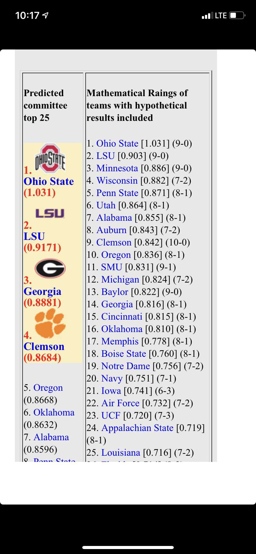
Today is a big day in the life of my college football playoff predictor site (playoffpredictor.com). Today is the second CFP committee ranking for the 2019 season, which means it is the first prediction week for the computer model.
what is in store for tonight? According to the model we will have Ohio State, LSU, and Clemson in three of the four spots. No surprises there. One surprise that the playoffpredictor says that differs with the AP committee poll – Georgia, not Alabama is in the fourth slot.
Personally, I think they will put Oregon in that slot – I think they will consider a last-second lost to Auburn on a neutral field much superior to a loss to South Carolina on Georgia’s home field. The problem with the first Prediction of the season is that there is not much bias information, those biases tend to smooth out as the season goes on.
If I were a voting member of the committee I would advocate for exactly what the computer says, which is Minnesota and Wisconsin in spots three and four. No Clemson, no Alabama, no Georgia. Minnesota is obviously unbeaten, but I just don’t see the committee changing on a dime from Voting them 17 to voting them number three. I hope it happens, but I’m not holding my breath. As far as Wisconsin? Well they were destroyed by Ohio State, but Ohio State looks fantastic. Other than that just a one point loss to a decent Illinois team. That certainly just as good or better than anybody else’s one loss who has some quality wins to go along with it. Alabama has nothing in the terms of quality wins. Their best win is Texas A&M, followed by Tennessee, southern Mississippi, and Duke. Yes, Alabama’s second best win was to a team that also lost to an FCS level team this year at home. Ouch.
Stay tune for 7 PM tonight, when we see if the first prediction is 75% correct or 100% correct.
5 years of college football data are in the books and I have enough data now to look at the playoffPredictor biases and make some determinations about habitually overrated and underrated teams that the playoff committee loves or snubs.
A little primer if you need it — each week of the college football season the computer assigns a rating and ranking to each top 25 team. During weeks 9-15 the playoff committee also assigns each team a ranking. Each week we can compare the committee rankings to the computer rankings and make an objective determination about over-ranking or under-ranking.
Using final season average rating biases, here is what we have after 5 years.
Conclusion? The perennial over-ranked team are also the teams that most often make the college football playoff. 3 out of 5 years for Alabama, Clemson, Washington and Baylor. 4 out of 5 years for Oklahoma and Mississippi State.
Interestingly, Ohio State (the only team besides Alabama, Clemson and Oklahoma to make multiple playoff appearances) has zero seasons over-rated or under-rated by the committee.
But there you have it. Conculsive proof that the rich in college football get richer, not because they are better, but because us humans are biased to think of the bluebloods as better.
I am a very fortunate person. Besides being blessed with a wonderful wife and family, I get to work for one of the greatest companies and brands in the world, Cisco Systems. One of the best perks of working for Silicon Valley companies in sales is the annual sales conference. Ours (rebranded this year from GSM/GSX to Cisco Impact) was once again a fantastic experience for me and I am leaving Las Vegas energized, proud, and ready to blow out our region quota.
I had two goals going into this week- I wanted to meet two people:
#1 – Kelly Kramer, CFO of Cisco Systems
#2 – Miyuki Suzuki, EVP of Cisco Asia Pacific
As most people who read this blog know, I am going back to school to earn my MBA. It is my stretch goal that about 7 years from now (when my girls have graduated high school and I have finished my MBA) I can get a job in either New York or San Jose doing corporate finance and strategy work – very different from Account Solutions Architect work in Oklahoma. I wanted to meet Kelly and see if she had any advice for me in that career path. I did see her Wednesday night at the Presidio event at Drai nightclub, but I felt that was too loud and not the right time/place for a career advice talk. Probably my loss. I do however have a backfill for that miss – I met and talked with Tom Koppelman (CFO, Americas Sales) at the Americas Advisory Council reception on Monday evening. Tom was generous enough to give me his time and advice. He even sent over John Moses (VP of Americas Partner org) to meet me and pick my brain on Cisco owning state contracts vs partners owning the contracts. It is certainly nice to feel heard at that level.
For the 2nd meeting I did stalk and meet Miyuki after her APJC session (yes, I skipped my own Americas session to do that). Dr Margaret Shaffer of OU is taking about 30 full time MBA students to Singapore this January, and I promised her that I would give a Cisco executive corporate visit in any country on earth she wanted to go to. Miyuki is boss over about 6,000 people and she has a great story to tell about growing up in Australia to leading JetStar Japan to EVP of Cisco Asia-Pac. The students I know will love talking to her about what business in Asia is really like and (they better) give her some feedback, some learning that makes it worth her time. Why I feel so motivated to build a bridge from the OU business side of the house to me I don’t sometimes know when I see the IT side about to deploy a bunch of Aruba APs in the stadium, but I have a deep desire to be a true partner to my customer, not a supplier. I keep plugging away and trust the process.
With those goals out of the way let’s talk overall conference themes. The theme this year was “Be the bridge”. After all that is what Cisco is. We connect. We build bridges of the technical kind. We connect people, ideas even cultures and really move forward the world. It is something to take deep pride in.
This is Eileen. Eileen was one of the 98,000 people on the streets on San Jose homeless. Homelessness in San Jose is a chronic, shameful problem for a city that is so rich, and Chuck Robbins (our CEO) is taking a personal responsibility to do something about it. Cisco built apartments for over 100 individuals like her and gave her a key for the first time, giving her pride. Such a powerful thing we do.
We also celebrate last year’s success at Impact. Last year Cisco grew revenue year/year at +7% — which does not sound like that much, but actually is the best growth since FY12. In fact, this fiscal year we crossed $50B in revenue for the 1st time ever (yea!). We have the largest cybersecurity business in the world, at that’s growing at >+10%. The stock has doubled over the last two years, but really flat over the last year. I do think Cisco stock hits a new all-time high above $80/share sometime in the next 2 years, unless there is a recession. Unfortunately, I am more beginning to believe a recession will happen. This week the 2-10 yield curve inverted. Not good at all. I will feel a lot better after the 2020 elections are over.
We are moving more and more of our business to software. Gerri Elliott’s priorities for FY20:
1) Take market share
2) > 50% of overall revenue from software and services
3) > 66% of software revenue from subscriptions
Now on to fun!
We had Malcom Gladwell come on stage and talk to us. It was one of the more provocative talks I have heard at this conference, and probably will stick out in my mind just below Peter Diamandis’ talk in ~2015. Malcom made a point about weak-link organizations (soccer, medicine, and Henry Rowan) and strong-link organizations (basketball and John Paulson). He talked about how the world needs more weak-link thinking. Interesting. I’m not sure I agree with him, especially in a sales organization. I thought it was funny, even though he pontificated about the world needing more weak-link thinking, he seemed to imply his magazine (the Atlantic) was a strong-link place, and he was the strong link in the magazine.
I found it interesting he was talking about philanthropic giving and he is truly shaping people that can make a difference to the next generation. Chuck Robbins is doing fantastic for the company and he is getting compensated commensurately. Somewhere in the neighborhood of $20 million per year. I can easily see after 10 or more years at the company at CEO he will be in a position to donate that $100M gift. And if he chooses strong or weak link, Gladwell will have shaped some small part of that.
Then we brought Sting in. He sang 2 songs unplugged and acoustic (Message in a bottle and Every breath you take). And talked about his passion. I found it interesting that he wrote Message in a bottle back in 1974 and everyday people want him to sing it – how does he keep that passion? How does he keep motivated? He talked about his job being to sing with “the same passion and curiosity” every day. He finds something incremental each time he sings, and it keeps him going. Another Sting quote “We cannot just build a wall around ourselves, we need to bring up the weak-link people”. Seemed to be a theme from all entertainers, and perhaps they are right. I was impressed with the respect Sting showed for his wife and her compassion for women at the border and claiming political and economic asylum.
Then there is this guy from Cisco Japan, who runs a whole marathon in 2 hours 45 minutes. Wow!!
So this year the closing act was Pitbull. Great show! Even though he did not play Timber, wow – he put on a production with Give me everything and Feel this moment. Fire, compressed CO2, confetti – and fantastic dancing. For a guy he can really move his hips.
So this year I decided I would get to the arena early and get on the front row, both for Gladwell, Sting, and Pitbull. I’m very glad I did. The region manager met and had a dinner that most attended. I’m sure the shrimp was good, but where else can you get a front row seat to talent like above? It is a fantastic opportunity. I’m humbled and thankful to get the experience. I never take for granted the army of people that dress up and serve me at this event. Thank you Cisco!
For ten days in May 2019 I was transformed. Not an accidental or surprise transformation, but the result of an intentional effort to be transformed. Of course we were thousands of miles away from home, but that was only a small part of the story. Before leaving Oklahoma, I put on a telling out of office message on my work email – “I will have no access to email”. Work calls to my cell would go to voicemail and not be returned. Ten days would be the longest I have ever been apart from my wife since our marriage. The apps that I normally use on my phone like reddit and yahoo finance would not be used. I was going to do life differently and see what came out on the other side.
This report details the results of my group trip and what I learned about business and culture in North Asia.
Expectations
One of the first things I learned happened before I left on the trip. For some reason I had believed (incorrectly) that a country’s economy could be grouped in developed and developing – only 2 classes. There are in fact 3 classes – advanced, emerging (the BRICS countries), and developing. My expectation was that China would be poor and cheap and that is mostly what I experienced. My expectation for South Korea was that it would be rich and expensive and internet access there would be off-the-charts fast, but I found prices to be moderate, and the internet no better than the internet at home. In short, I saw little differences between the emerging economy of China and the advanced economy of South Korea. Of course, Beijing is not China (as stated eloquently by Alvin) and I would love to take 2-3 months to really see China. However, I can only write about what I experienced myself.
What follows is a chronological listing of the events I experienced and my thoughts about them.
Thursday May 16, 2019
I left home at about 3pm. My flight path for the day would take from OKC to LAX, and then from LAX to PEK. I decided I wanted to take a flight Thursday afternoon and get to Beijing Saturday morning, which means crossing the Pacific at night. This is different than the conventional way to travel, which would be to leave first thing Friday morning and get to Beijing mid-afternoon on Saturday. I figured the days abroad were precious and few, so stealing one additional day instead of letting it go to waste with travel would be the way to go. Fortunately, Kaydee Cunningham was with me on this logic so I had a travel-mate.
One of the fringe benefits of the whole experience was getting on a group text string with the other three PMBAers from my cohort – Kaydee, Ashley and Angela. From May through March we communicated nearly daily about our expectations and desires for the trip. As a guy that does not get that many social texts, what a thrill that was in itself. Kaydee booked on the same flights with me. All four of us should have been on the same flights together, but I booked without confirming from the other 3. It turned out that Ashley had points to use on American and booked on American. Angela followed her lead. So instead of the four of us traveling together it was 2+2. Angela and Ashley would have followed me and all four of us would have traveled together if I was clearer in my communication and had the empathy to understand and serve the needs of this group. This character flaw I came to see in myself would become a recurring theme for me – one that I really dove in to in South Korea.
We had a six-hour layover in LAX – as far as I’m concerned far too long to kill in an airport, so we rented a car and drove for some Mexican food (Sol Mexican Cocina). I got to know Kaydee a bit better, ask her about her and Tyler’s OSU roots. We drove back by 10pm for a 1am flight. LAX was so crowded. The drive from the Mexican place back to LAX was quick enough, but the shuttle bus from Hertz back to the terminal took an hour. Good thing we were planning on arrive at the airport 4 hours before the flight. That meant that the slow ride back to the airport was not stressful. The flight ended up getting delayed to 3am anyways. As a side note, when I refilled gas for the rental car I paid $5.10/gallon. Yikes, the cost of living in California is high.
The flight ended up being very good. The airplanes for overnights from LAX to east Asia are not an every seat filled proposition, as are the flights during the daylight hours. Kaydee and I had three seats for the two of us. Not first class, but not too shabby either.
Friday May 17, 2019
This day did not exist for me. Technically I had three hours of this day as we waited in LAX till 3am for our flight to leave, but such is the reality of air travel across the Pacific. Two days to get there, almost no time lost coming home.
Saturday May 18, 2019
Kaydee and I arrived at the airport around 7am. I always get window seats when I travel, and from the air I noticed a lot of blue roofs over Beijing. I can’t say why those blue roofs are there. The only other place I have seen so many blue roofs was Haiti, which I landed about 1 year after a major earthquake and there was still much temporary housing on the island. These blue roofs looked different to me though – solid construction. I’m still not sure what all the blue roofs represent.
My expectation was for the Beijing airport to be modern, clean, efficient- and it generally was. My preconceived notion is that infrastructure in the USA, especially around the east coast of the US, is dilapidated and old, where infrastructure in East and Southwest Asia is clean and modern. I’d say that held true here. I was surprised we were forced to give our fingerprints (digitally, of course) upon arrival in Beijing or else there was no entry into the country. My first act at arriving in China was to pull out Google translate and give it a try. It labeled the first sign I came across to read “foreigners fingerprint buffet”. Funny, but good enough for me to get the gist of what I needed to know. I learned after arrival that a new airport in Beijing is under construction and will be opened later this year. If the current Beijing airport is the worst of the China airports that it needs to be replaced then China has hands down better airports than the US.
One app I had ready on my phone was Didi taxi. There is no Uber in China as China promotes their own enterprises that have state backing. I used Didi to pick up a taxi and take it straight to the hotel. That worked flawlessly. No need to explain or translate anything for the driver – he took us straight to the hotel. As a bonus we got to drive by Tiananmen Square and the forbidden city along the way to the hotel. I could see, and snapped the picture of Chairman Mao.
Upon arrival into the hotel our rooms were not ready. That was not unexpected since we were so early. The hotel did hold our luggage and give us access to the spa where we were able to take showers after the long transpacific flights. The spa was first rate – large, clean, several hot tubs with hot water (even though no one was there but me). The pan-pacific Beijing was definitely a five-star hotel, and such a reasonable price. It was nice to see PPP work in my favor – very much the opposite of having lunch in Switzerland. One of the things Kaydee and I wanted to do with our Saturday was ride bikes around the city. When I was last in Beijing (1978) there were very few cars – it was all bicycles. I am happy to say that even though there are many cars in Beijing I still saw many people on bikes. Perhaps older people, but the point is the bicycles have not gone completely away. I’d say 90% of traffic is cars, but 10% is still bikes, based on what I saw. We were told by the concierge at the hotel to go to a place in southern Beijing named Fengtai to rent bikes. After a 30-minute Didi ride we were dropped off in Fengtai and it was a dump. We did not even try to rent bikes there, we just hopped another Didi and got out of there. By the hotel I noticed many bikes for rent via iPhone app. There were many Mobikes all over the place which would have been perfect for Kaydee and I. Unfortunately, I could not rent them. I could download the app, but to add payment to the mobike required a mainland China bank account. I even tried later in the week to open an account at Bank of China, but I was denied (can’t open it on a tourist visa). So, no bicycles for us. I would later learn a phrase from some of the other students at Tsinghua University: “TIC” which is an acronym for “This is China”. You should not have the expectation of friction free life.
So after our bike debacle, we took a Didi back to Beihai park. We walked for about a mile and it was a decent diversion. I think we were trying to find a Chinese bustling market scene, but the park was fine. We did notice some people dancing in the park. For lunch we found a street restaurant. Kaydee did not care for her food, but mine was fine. I remember lunch and a beer was somewhere around $3-4 US. Nice! We also made a few minutes to see the giant panda at the Beijing zoo. Cute! Checked that off the list and went back to the hotel to await the arrival of Angela and Ashley.
That evening Kaydee’s cousin recommended a restaurant named Dali Courtyard. That was my favorite meal of the whole trip. It was a restaurant in Dongcheng. Several things were memorable about the meal: First off, getting there – again Didi taxi took us to the area, but the restaurant was not on the main street. We had to go down the alleyway, past the walls of the Hutong and turn a corner. We are all doing this as we are blindly following directions on a phone. Amazingly it was correct! The meals there were fantastic – they just start brining you plates. Plates after plates and more plates. It starts with light appetizers and builds to fish, and main courses. You are outside on a patio under the moonlight. Candlelight, perfect temperatures, abundant and inexpensive well prepared food and the company of 5 PMBAers (myself, Alex, Angela, Ashely and Kaydee) – what an experience! There must have been 20-30 courses during this meal. Amazingly, it would become a theme for Asia dining.
One other odd thing – I had no idea who my roommate was going to be – but the night came and went with me alone in the room. I have never had a roommate in my adult life. The last time I had a roommate that was not my immediate family I was 12 years old in summer camp. I was very apprehensive about the whole roommate thing, but I guess if you are going to be a student you get the full student experience J. Only later would I understand the struggles Adam was going through to get to China. Takeaway – If you are going to take the nonstop from DFW to East Asia, just drive to DFW. Don’t bother with the flight from OKC to DFW. It just is not worth it. Really though, I like what I ended up doing. Nonstop from OKC to LAX, a six hour layover in LAX (you want to give yourself time for airline delays), and then a nonstop from LAX. I think that is the best way to go.
Sunday May 19, 2019
The morning of May 19 I woke up early – probably 4am. In general, when I travel I don’t sleep much, and this trip was full of adrenaline. Each day of this trip I only slept ~4 hours per night. I got out of the room and walked to the subway. The subway was clean and empty this time of the morning. I also walked by the local schools and the local 7-11 equivalents. I tried some bizarre boiling seafood at one of the 7-11s. At least I think it was seafood. I only ate one ball and disposed of the other 2 balls on the stick. Since I had not had a hepatitis shot I did not want to get sick on day 1, but in general I don’t feel I have a weak stomach. The local food looked too much like home food at 7-11s – Doritos, Pringles, etc. I walked back to the hotel and hot ready for our group trip to the Summer Palace and the Great Wall.
At the Summer Palace I was taken with the architecture. Especially the roofs, which have this beam and post construction. Where the beams support the rafters, the beams are sloped – not straight. This was common in Korea and Japan as well. I found it pretty, and the amount of detail artwork that went on and on in the palace was impressive. Many of the tourists I noticed were Chinese – I imagine Chinese from other parts of China. My expectation is that 20 years ago the tourists were mostly foreign, but that was not the case anyone.
I was also very happy with the amount of English on signs at public places. One that caught my eye was at the exit of the palace – written in English – complaint department phone number. Can you imagine us putting a sign in Mandarin next to Abe Lincoln’s memorial that says “If you have complaints with our memorial, please contact this number and we’ll be happy to help” Of course not! The culture of service in Asia is remarkable.
Next we went to the Great Wall. On driving to the Great Wall I paid attention to see what the road (infrastructure in general) was like. One thing that caught my eye was a massive elevated road under construction that ran parallel to the existing highway. Even though their existing roads are not terribly crowded, I can tell the Chinese government is making investments in new infrastructure. When is the last time we had new Interstates? Or even an expansion of, say, I-35? Leave the current road in place and build a new 6 lane highway parallel to it that runs from Norman to Dallas – leave the 70 MPH speed limit on the old road, force 18 wheelers to use that road only, and design a new road that can handle 120 MPH speeds safely. That kind of investment in infrastructure in the USA would pay long term dividends for our country down the road, but it seems like we don’t have the leadership with vision anymore like we did in the 1950s.
I found the Great Wall to be a thrill. It was so uneven and up and down, I cannot imagine how horses rode on the wall. At a couple places I needed to get on all fours to go up and down the wall. I was determined that I would walk all the way to the end and back, which I did. I’m not quite in the shape of the twenty year old people on the trip, but I’m not bad either.
Monday May 20, 2019
The first corporate visits were to be later today. I got out of my room about 6am and walked around. I saw the kids entering their school (“The experimental highschool (sic) attached to Beijing normal university”). All the kids had on school uniforms. I also noticed the younger kids (elementary age) also had on uniforms.
Visit 1: Tron Space
The first corporate visit was to Tron Space – a company incubator in Beijing. It struck me that this was very similar to what I would see for technology incubation spaces in the US – shared, common high-tech companies. First Dr. Jessica Hao (from the school of Economics at Tsinghua University) explained how there was $20B USD in venture capital available to the companies in the area. Then, our presenter was Mason from NavInfo – a mapping company with 4,000 employees in China. Their story sounded like any capitalist story back home – a Toyota partnership started in 2002, a listing on the Shenzhen exchange in 2010. One thing I found interesting was the State-owned enterprise facet of the company – another company called China Survey owned 10% of NavInfo. I asked a question about what the Government of China intends to do with that stake (sell it, etc.), and the answer was no- that is just a part of doing business in China. You just have a long-term government partner / ownership. Tencent owns 10% of NavInfo – and it is common that Tencent and Alibaba are the early series funding for their high-tech IPO industry. So for NavInfo:
Tencent owns 10%
China Government (China Survey SOE) owns 10%
Management of NavInfo owns 10%
Public Investors own 70%
That structure is not unlike capitalism back in the US, with the obvious exception of the 10% government stake, but considering how nationalized our banks and auto industry became in 2009 I guess it is not the different either. I digress.
Mason did mention that 30,000,000 new cars were sold in China in 2018 and for 2019 he expected that number to drop – not to slow the pace of growth, but an actual drop. I asked if we should infer from that drop that the Chinese economy is growing much less than the 6% currently believed, and he said no – it’s about making strides against pollution. I guess we were lucky, there was a big rain shower the previous night and I had no problems with pollution in the air. Angela got us masks to wear like 10% of the Asians do (they wore these masks in Korea and Japan as well. Heck, one person danced in a club in Seoul with a designer mask on), but we never needed to wear it – only for fun. Still, I’m not 100% sure I believe him when he showed no fear for the Chinese economy. I could sense they are all very nervous about the trade tensions. Mason did mention that 54,000 cars sold each year are EVs, and if you want an EV you can get one right away, where if you want a conventional car there is a 3 year wait for the license. That’s definitely not capitalism, but I’ll give them a pass due to their pollution problem. I give them credit for getting serious about their problem and owning it. Mason himself did not own a car, instead he had a driver. Why bother owning a car when you can have a driver instead?
My final note from NavInfo was “Data and Algorithms <- that’s what it’s all about”. And I can guarantee that exactly what it’s all about for similar companies back in the US. Indeed, I found many more similarities between businesses operating in China vs the US than differences.
Visit 2: Tsinghua University
The second corporate visit was to Tsinghua University. Hao Chen gave us a fantastic overview of culture and China. I take away a couple points from her (fantastic) talk – like China has 829 million Internet users as of 2018, so still another 400 million people are left to connect – which means to me there is still room for growth in China. But what I remember there was #1 getting coffee with Emma and #2 the University tour.
For coffee, during a break in the lecture we tried to go with the students from the other visiting university to a Luckin coffee around the corner. Luckin was interesting. You could not order at the counter. You could only order using an app. You could not pay in cash, you had to pay via app. Of course, since Alipay and WeChat pay require a mainland China bank account – I could not order coffee. That’s when I learned the phrase “TIC” from the other students that I discussed previously. I saw so few people in the store, but so many coffees on the table – all internet app orders. The barista at the counter took pity on me based on my google translate skills and handed me their phone which I gave to Emma to figure out how to order her latte and my Americano with an all-Chinese app. Well, she figured it out, I payed the barista yuan cash I had with me and the two of us brought our coffee treasure to the class.
For the university tour it came out that tuition there was peanuts – something like $800USD per year.
One other bonus at Tsinghua – they had Eduroam configured and I was able to get on their WiFi using my OU credentials. How cool is that! In fact I looked at many place to see what the WiFi provider was and it was Cisco access points in almost all locations, the only place I saw Huawei was at the Beijing capital airport. Other than that all buildings had Cisco infrastructure. I find that fascinating and amazing.
That night we went to the pants building for dinner – and my Asia drinking was officially on. I’ll bet in the past year I have had a total of 5-6 alcoholic drinks, but each night, especially in South Korea I had 5-6 drinks per night! I loved every minute of it!!
That night was the series finale of Game of Thrones – I remember watching it from 1am to 2am in the room with Alex, Angela and Nic. What a bunch of fun nerds we were!
Tuesday May 21, 2019
I don’t think I slept at all this night. I may have lied in my bed, but too much adrenaline. It was too weird with a roommate next to me (Adam finally got in from his marathon journey). I think I showered and left by 4 or 5am. I told Adam that I would see the great wall with him because he should not see it alone, but as it worked out I did not go with him (that would have made him uncomfortable, which I totally get). Instead I woke up early in the morning (I actually never slept) and decided I would find the Cisco office in Beijing and call home with telepresence. I had to be back at 8:20 for our ride to GE Healthcare, and I left the hotel by 4:30am. I took at DiDi to a place I thought was Cisco. It was not, but the guard there went out of his way to help me into any part of the office building I wanted to get into. Again, very surprising and a different culture than the US. I realized I was in the wrong building and took another Didi to the correct building, and my id let me in. I had the telepresence and I found it no different than doing telepresence from Kansas City to OKC. The speeds were fast and natural. The office culture at Cisco Beijing looked very much like the culture at Cisco USA, based on the design of the building, the free snacks, the telepresence rooms, the audio privacy rooms, etc. I hung up with my family at 7:20am and had to get back to the hotel by 8:20. It was only 5 miles away, but I learned something that morning – Beijing traffic does not move at rush hour! My Didi driver explained to me that if I needed to hurry I should take the subway, so he dropped me off halfway through my ride and I took the subway and ran from Xian station back to the hotel, with just minutes to spare I made the bus. It’s amazing what I feel I can do with the technology in my hand in the form of a phone – mapping, translation, subway navigation. I feel like a superhero in a foreign country with it. Take it away and I’m a lost idiot.
Visit 3: GE Healthcare in China
I took back a handful of things from this visit. GE Healthcare had a similar ownership structure to NavInfo, where there was a SOE that was part owner in the enterprise. The visit confirmed for me the growth area that China is. ~3,600 urban hospitals (which can be considered developed), but an additional ~80,000 rural hospitals (which are developing). The rural hospitals deal with lack of electricity and clean water as issues, very 3rd world problems. The growth GE Healthcare has in China has been ~15% per year, where similar products in the US at ~1% per year.
I did hear from Joy (runs supply chain management at GE Healthcare China) that they are shifting some of supply chain to the US due to the trade war. My takeaway on that is that the Trump tariffs are working, even though I understand the policy is hated. I feel it is hard for Americans to separate the policy of Trump from the person of Trump. I feel overseas they don’t like Trump, but they respect him as a US leader, and hope they would have a leader that fights for their country like they perceive Trump fighting for his.
Another takeaway from GE Healthcare that took our breath away was the term 5/10/7 – meaning working hours of 5am to 10pm, 7 days a week. That equates to 119 hours/week. Their culture is engrossed in “work” in a way we can’t comprehend. Of course, their work includes meals and events and activities, but setting a standard that high is insane. I get it that companies can get this kind of culture because if someone slacks off there are 30 people on the street to replace that person, but still this expectation is staggering.
A nugget I picked up at GE Healthcare came at the end of the meeting. We were extolled: “You know how me work. Now, learn how we think. Go to a church.” That was my favorite line from all of Asia. I never did go to a full church service, but that is definitely something I would do during a future extended visit to Asia.
Visit 4: Goldwind
Before getting to Goldwind we had some time to kill and the bus dropped us off at some non-descript mall in south Beijing. Something near the Guorui Group Ronghua World Hotel. This place shocked me. It looked bigger than citycenter in Las Vegas, but it was just some other area in China. I’m thinking if this place was in the US everyone would know about it. It is amazing to me the growth and development in China.
Goldwind I took no notes on. I found the exercise room and greenhouse interesting, but it just means the management of Goldwind likes these activities, nothing special. I find it odd that in China basketball is such a popular sport, but we know nothing of their local leagues. In fact, our guides favorite team was the Miami Heat. How all these Chinese people prefer US basketball where the games are played in the middle of the night their time and teams that they can never possibly hope to see in person – it baffles me.
Farewell dinner / I think no staying out that night.
Tuesday May 22, 2019
This morning we saw Tiananmen Square and the forbidden city before leaving the country. There was such a long line of people to see Mao’s mausoleum. I would have absolutely loved to see that, and also see the sunrise flag ceremony, but I guess that a reason for me to come back. I was fascinated with the line of Chinese that come to see Mao’s body. The line was thousands of people long.
The forbidden city evoked incredible emotion in me. I had been there before, when I was 8 years old with my parents. It seemed all weird and wrong to be there without my family. Emma took great pictures of me with her nice camera.
One thing that is fascinating about the Forbidden city is the stone carvings. There are beautiful, ornate stone carvings all around with what once was detailed artwork, but the acid rain has melted these carvings. I understand why the Chinese are sensitive to pollution.
On to South Korea
I loved South Korea. By this time the group was bonding well, and our partying was fun! The lights and street scene in Myeongdong were wonderful. Something had changed in me by this point. I was determined to be different in South Korea. I felt I was too much like “rain-man”. I wanted to be natural, less aggressive. I was determined I would keep quiet and let others talk during the company visits.
Wednesday May 23, 2019
Visit 5: DreamPlus
The obvious comparison is between DreamPlus in Korea to Tron Space in China. Again, more similarities than differences. My takeaways from the DreamPlus visit were:
Lots of people in shared office space – I saw no one working in private offices. I take this to be the Asian culture.
The person on the 3rd floor next to the library was literally asleep in a chair facing the window. I am surprised that is culturally accepted at work in Asia. As strange as it is to say, that could be culturally accepted in the US, so again, more similarities than differences.
The access points in the DreamPlus space were also Cisco Systems. It is very encouraging to see our global presence. WiFi is very important and I would argue part of a society’s culture, so again more similarities than differences.
I also learned at DreamPlus that Christianity is a very popular Korean religion – the estimate from our host was 25% Christians, 20% Buddhist for Korea.
I loved the basement of the DreamPlus space and that showed the influence of Steve Jobs. The quote in pink neon of “Stay foolish, stay hungry” – even in a basement of Seoul.
Visit 6: PNG corporation
PNG was an eagerly anticipated visit for me. The reason is one of my very good friends in Norman is Scott Shuler who is president of Top of the World caps. I have known both Scott and his business partner Pete Wilson for 10+ years, and I know their partner in manufacturing in Asia is Harold Koh.
Initially, the things I took away from PNG were more numbers and facts instead of culture. In particular:
PNG Vietnam produces approximately 1,000,000 hats per month
PNG Vietnam employs approximately 1,300 workers
The PNG embroidery machines run 24 hours per day.
This is a labor-intensive business
Each embroidery machine (imported from Japan) costs $100,000
They have 100 embroidery machines on the floor
Basic math tells me that if the margin on hats is $5 that’s $5,000,000 per month for 1,300 workers, or an average of $3,800 per month per worker. I learned all 1,300 workers cycle between all 3 shifts (no one person gets only the day shift and no one person gets only the night shift). This is different than American culture where a person would only work the day shift as a full-time job, but get paid less than a person who only works the night shift exclusively. You can see here the culture of shared labor fairness in Asia.
At $100,000 x 100 = $10M in capital tied up on the floor. The carrying costs for $10M at 10% and 10 years ~= $150k per month, so that is fairly low in comparison to the labor costs per month. So, it would seem to me that running 3 shifts 24 hours is more of a culture decision, not a capital decision.
Harold did lament that manufacturing wholesale prices have risen only 5-7% in 29 years, even though expenses have increased more than that, so his business has gotten squeezed over the years. He sees an oversupply situation. He would like to move the business from college licensed headwear (where there is more competition) to corporate brands (such as Dickies) where there are lower minimum requirements.
Things I learned at PNG:
One takeaway I had from the canned PNG briefing and the PNG presenter is I could tell how they were trying to impress on us their social conscious labor practices. They mentioned it several times. I would have no reason to assume they were anything other than above board with their labor policies and people; I found it interesting they wanted to bring that conversation up.
After the first couple of Q&A (directed to the presenter) I asked a question for Harold. After that, all Q&A were directed to Harold. We wanted to talk to the founder, not a corporate spokesman!
I also find it neat that Harold and Pete met and formed their partnership at a trade show. For as much as we complain about trade show floors and the drudgery of it, the reality is that’s how and where transformational business happens.
Adam asked a question to Harold on what his management philosophy was. Harold responded with that he wants to impart western philosophy into his east Asia business. The irony is palpable: we are going there learn Eastern philosophies, but he is trying to get our philosophy. The world has indeed become a very small place. His particular B-School philosophy boiled down to 3 components:
Pick a target
Narrow the focus on that target
Dominate the market
That night was a fun night from a drinking / clubbing point of view. We even finished the night at a karaoke bar. Fun thrill!
Thursday May 24, 2019
Visit 7: Taihan Textiles
I very much enjoyed the Taihan factory tour. I cannot imagine going to Asia on a business school trip without any factory tours, so I am very glad we got this one in. At Taihan I learned there is a $10 / hour minimum wage in Korea and that 52 hours per week is the normal working hours. $10/ hour is obviously more than labor in China, and I heard they were viewing the trade tensions as an opportunity for them to compete with China better, and take business from China. Again, another perception of mine that the trade tariffs may be good and right for the US right now.
My goal going into Taihan was to simply sit down and be silent. I did not want to be dominating the conversation. That is annoying to all. I don’t want to be that person.
By this time, I had become hyper sensitive to changing who I was at these meetings. I started to note my failures. I came out of the meeting with the following scorecard:
I know these seem silly to others, but I see these all as significant failures that I want to address in my life going forward.
Visit 8: Korean Embassy
Here I wrote down every question asked and who asked it. I found out I love doing that! It helps me understand the people around me and what their care about are (empathy) and it prevents my mind from asking excessive, stupid questions. That’s a practice I want to consciously continue next year in my MBA classes.
I went in with a challenge to myself of not asking any questions. Of course I failed, but my scorecard was cleaner:
We heard from Bo Miller (a career foreign service officer) and Cameron Jones (the North Korea economy expert for the US). I very much liked the style of Cameron Jones. Very thoughtful, thorough and respectful to the audience. He was our groups favorite speaker.
Angela asked a question about the North Korean defector that Trump introduced at the 2017 State of the Union. It lit up Cameron’s face and drew a passionate response from Cameron as he stated that that person had been in this very room. I could tell Cameron was lighting up for an audience that gets it and is worthy of his time and energy. I totally love Angela as a leader and I would be happy to follow her anywhere. I respect her mind and her abilities.
Seth asked a question about how to get contacts at the department of commerce and US-China trade tensions.
Adam asked a question on the culture of business in Korea. I found Adam’s questions very insightful – he was very intentional bout applying the lens of what can the US learn from East Asia, not just in what people do but in how people think (and should think).
Dr. Shaffer asked a question on economic vs political defection from N to S Korea
I asked a question on groupthink – having had the same N Korea policy for so long without real knowledge of what happens there. I got the 1 failure tick for that question.
Angela asked another question about Reunification vs Denuclearization. Cameron made it clear policy one of the US is denuclearization. He also gave insights the old South Koreans are for reunification, but the young South Koreans are against it. They don’t feel they should have to pay for the previous generation’s mistakes.
That night we went back out to go drinking, but I turned in early. Couldn’t do the last full night. I took 3 of the undergrads back with me and bought them ice creams at McDonalds while the older PMBAs went back to the same club from before. There Angela met a couple guys who said they were with Trumps security detail and Trump had been at the JSA DMZ the previous day and that’s why we could not do that tour on that day.
Friday May 25, 2019
Korean DMZ
Trump in S Korea and Tokyo at same time
Saturday May 26, 2019
Japan
This is where my reflection ends. I met Shelli at the Tokyo Haneda airport, and at that time this trip transformed from a group activity to a couple’s trip. I did not anticipate that happening, but I get it. You can’t force friendships. I enjoyed Japan, but not in the same way I enjoyed China and South Korea.
In Japan I did love the hotels Dr Shaffer put together – staying in the bright lights of Shinjuku was excellent. Being in Kyoto at the Torri gates and Steve Jobs’ favorite temples was fantastic.
Final thoughts:
I did this trip at 48 years old. I realize this is a trip more for 21-year-old kids, but I loved it. I appreciate Emily Kuenzi telling me that this trip was for me and it was OK for me to be there. I get that doing something different does invite the questioning of motives and character from others, but I can’t worry about others. I really appreciate the PMBA school making this trip available and I sincerely hope in the future enough PMBAers in their 30s and 40s will come along to make this a PMBA only trip. But honestly, I loved doing this with undergraduates. As a dad to a 20-year-old kid at OU now I felt that I could relate with the undergrads better than the 35-year-old PMBAers. I took full advantage of this in South Korea when I asked AJ and Jake to dance to “I’m squidward” in front of a squid tank. I am sure the 35-year-olds could not get the reference, but I loved what Jake said to me “that hit me deep”. I know it seems silly, but I love that I can relate in a way the others could not.
One other thing I enjoyed was the fact that, speaking broadly, the PMBAers could spend money. As people with full-time careers, we had resources the undergrads do not have, and it was fantastic to spend it forward. I enjoyed Angela and I buying all drinks and food for all the undergrads at the Korean BBQ. I think it was $100 for each of us. No big deal to us, but a big deal to the undergrads J. When I think about it another way, I often look at my IRA balance and it is not uncommon for it to fluctuate by thousands or tens of thousands of dollars on a daily basis. So, while this trip was expensive, it was only expensive if viewed in the lens where I want it to be expensive. We are so fortunate here in the US and I see it when I travel.
On a non-Asia culture note, I was also struck with the difference in maturity levels and personalities from the undergrads. Take Riley – incredibly smart, 35 ACT, national merit scholar, moving to Dallas for Bain capital (L – I swear we export almost all of our good talent to Texas) and on the other side AJ – who may be brilliant, but all I can picture is his head engrossed in his phone reading science fiction even at the corporate meetings and farewell dinner. How bizarre to me! Unfortunately, my son is a friend of AJ and not Riley. But that’s OK – he has a good head on his shoulders and I believe he will find his place in life and contribute to society just fine.
I am very hopeful I get to do a trip like this again, or at least doing meaningful activities with the others in my cohort down the road. I respect these people at a business and intellectual level, and that is something special for me.
The 2019 OKC Marathon is in the books. This year Shelli, Austin and I all did the half-marathon. Results are back, and here is how I stacked up:
2 hours and 18 minutes to run 13.1 miles for an average pace of 10:33. My goal at the beginning of the year was to run in under 2 hours — well, that was just not going to happen. As much as I wanted to I couldn’t commit to the training needed to make it happen. Still, I’m happy with 10:33. I placed right in the middle for my division – place 156 out of 310 total runners male 45-49.
Since I’m into statistics now, I also calculated my Z score to see how I did against a normal distribution. The average finish pace for my division was 10:59 with a standard deviation of 2:28. That puts me at a Z-score of -0.18, which has a 1-probability of 57% . (In other words, I placed in the 57th percentile for my division). Not bad!
Here are the top, 50% and bottom finishers in my division:
Red skittles are scarce. At least that’s always been my impression every time I open a mini pack we get as halloween candy. Too many yellows, too many greens. Never enough reds. Possiblywrong recently published some data on 468 packs of skittles looking for duplicate packs. I wanted to use his research data to answer a different question: Are red skittles scarce compared to the other colors?
Using his data and the statistical analysis tools given to me by my MBA professor (Robert Dauffenbach) we can answer this question. First the raw data- in 468 packs of skittles there were 5583 reds, 5499 oranges, 5688 yellows, 5301 greens, and 5669 purples. Averaged out it is real close to 12 skittles of each color in a pack.
Close to uniform, but not exactly uniform. Let’s analyze this further:
From his raw data the standard deviations of number of candies by color is about 3.2. Here is the compiled data:
So, true population averages appear to be 12 candies of each color with a standard deviation of 3.2 per color (in one bag). Now the central limit theorem will help us here- even though the underlying distribution is uniform, a distribution of sample averages will be normal, assuming n is sufficiently large, and n=468 definitely satisfies this requirement (n>=30 is probably all we need to get from uniform parent to normal sampled means). Now if we make the assumption that the population means and standard deviations are 12 and 3.25 respectively, we can answer the question if the difference in Yellows (12.15) to Reds (11.93) is statistically significant. The standard error of the mean is the standard deviation over the square root of the number of samples = 3.25/sqrt(468) = 0.15. That means if we have have 12.15 yellows, that’s one standard error of the mean from 12, a result we should find 68% of the time. In other words not statistically significant. (Busted — yellows are not more common). Reds with a z-score of -0.47 are also within 1 standard deviation of the standard error of the mean meaning reds are plentiful — they are not held back, regardless of what I think.
However, the data does point to one outlier — greens. At an average of 11.33 that is -4.52 standard deviations below what’s expected. The probability associated with a z-score of -4.5 is about 1/100,000 — meaning if it was a daily possibility you expect to find it 1 day in 275 years. That is statistically significant and the null hypothesis that greens are filled at 12 per pack is rejected. The alternative hypothesis is accepted, and that implication is that skittles intentionally under-fills green in order to keep packs at 59 per pack and not at 60.
For my MIT class this semester we have to create a web site with at least 10 HTML forms. It should link back to a SQL database those forms can interact with. Griffin Pierce and I have chosen to do a project involving college football. We have a database of ESPNs play-by-play data for all college football games since 2002. Check it out, SaturdayCoach.com
Recently I finished reading the book Get in the Boat, by Pat Bodin.
The point of this book is that technical people are not in the boat with corporate leaders, because they speak a different language and have different priorities and risks.
Well, that’s nothing new.
However, the part of this book I found particularly enlightening was the treatment between technologists and IT. That hit me like a 2×4 square to the jaw. I got into this field 20+ years ago because coming out of college I saw with wonder the way Cisco Systems was connecting and changing the world. It was clear to me, even back in 1992, that people in the wake of Cisco Systems were the movers and shakers of the world, and only good things came from being associated with this company of strength. At that point in time central IT did not exist, not like today anyways, and central IT was being elevated — from a cost center to a strategic focus for the business. Very relevant. Somewhere along the way IT became a burden — divorced from the leading-edge technology that changes business for the better and gives each business who properly digests technology a competitive advantage against their peers and now married into a me-too table-stakes of basic uptime and SLA fulfillment.
For example, I know a VP at a leading higher education institution who has a main job of approval of emails that have to go out campus wide. Think about that for a minute- when did IT go from creating a project where a person in London could color-match a car manufactured in Berlin to bureaucratic email approver? And this is a vice-president. Makes you wonder how relevant the lowlife IT individual contributor is to the president of the University?
The book does a great job of understanding value-chaining: How can your actions at the Red level impact Blue, and impact Green. Don’t understand those colors? Read the book! It reinforces the basic message we already know inside – You are not relevant because of what you do, but because of how you affect other people.
When you talk to green about “technologists” they equate that word with blue people – lines of business who practice “shadow IT”. When you talk to Red about “technologists”, they will think IT. Big mistake. Even the way we as IT talk about Blue people is in a way to delegitimize and dirty them (again, shadow IT). We have to be those Blue people, not bash them!
For anyone who has read the Phoenix Project, this book is a great 2.0 read to that book. A lot of the principles and messaging connect.
This is a fantastic read for anyone who works in my field of technology, especially those who work or sell into information technology.
In my line of work (Higher Education) – we may have 5,000 full time equivalents in an organization. Of those, Id say Red is about 200 (IT people), Blue is 4,795 (faculty / staff) and Green is about 5 people. 5 People that’s all. A lot of titles like VP of applications may seem to the untrained eye to be Green, but they are blue. A teacher who is leading edge and consumes technology in her classroom in a way years ahead of her peers and gets better grades for students – Blue, not Red. I think of Red as lone-wolves in centralized IT. Period.